Honey flow between plates
I derived the discretisation and wrote a semi-implicit finite-difference solver for honey entering a gap between two plates, then checked the developed flow against the analytical solution.
Result
Simulated mean and peak velocity within 2.8% of the analytical profile at x = 0.723 m

Problem
Honey enters a 0.10 m gap between two plates at a uniform 0.05 m/s. Walls slow the fluid next to them, so downstream the flow should settle into the parabolic profile of plane Poiseuille flow, peaking at 1.5 times the mean, or 0.075 m/s. I wanted to model that development and check the solver against the analytical answer.
Constraints
- Newtonian, incompressible and laminar. The code treats 0.005 m²/s as the kinematic viscosity, which gives a Reynolds number of 1.
- No-slip at both plates, a uniform inlet and a fully developed outlet.
Design
The solver discretises the 2D Navier–Stokes equations by finite differences on a staggered grid, which keeps pressure and velocity coupled and avoids checkerboard pressure fields. It is semi-implicit: diffusion is solved implicitly as a sparse linear system each step, while advection and the pressure gradient are taken from the previous step.
Parts of the domain setup and implementation structure are adapted from an open-source reference by Ceyron. The semi-implicit solver, the discretisation and the analysis are my own.
What the solver shows
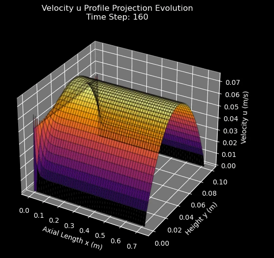
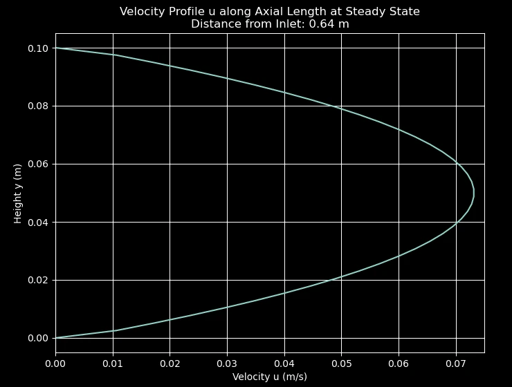
The three animations below come from the repository’s own run of the solver, not the rerun used for the numbers in Testing and results. The first two follow the flow over time. The third is a sweep through positions along the channel once the flow has settled.
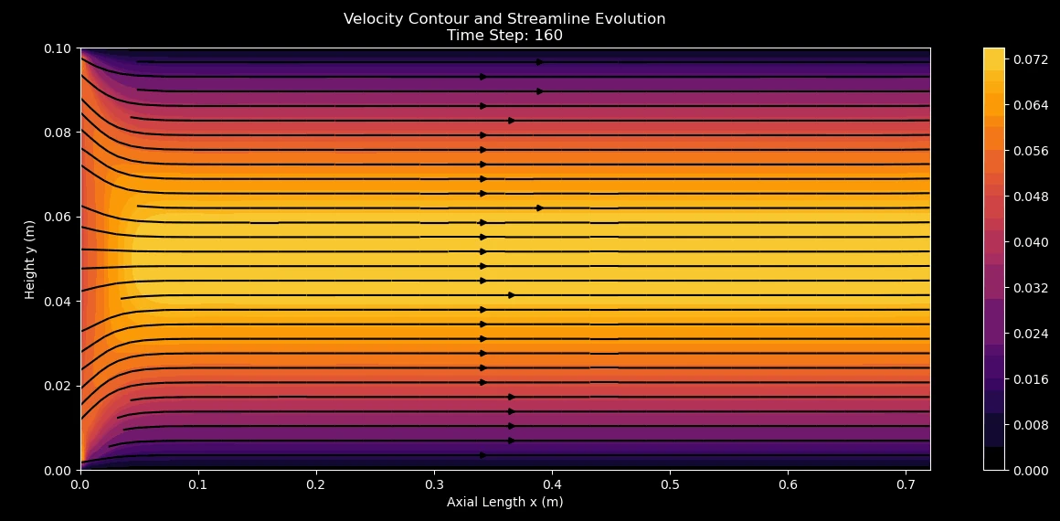
- x axis
- distance along the channel, 0 to 0.72 m
- y axis
- height above the lower plate, 0 to 0.10 m
- Colour
- axial velocity u
Testing and results
I compared the simulated profile with the analytical one at the solver’s downstream station, x = 0.723 m, at t = 0.160 s. Across 40 evenly spaced samples from wall to wall, the arithmetic mean velocity is 0.04870 m/s, 2.60% below the 0.050 m/s inlet. The highest sample is 0.07292 m/s, 2.77% below the analytical peak of 0.075 m/s. Both are simulation results compared with an analytical solution, not measurements.
These numbers come from rerunning the repository’s solver functions for the first figure on this page, with an equivalent conjugate-gradient solve of the same sparse systems. The repository’s README quotes 2% and 4%, worked out from its own reported values; the figures above go with the rerun.